Creating Urbanization Scenarios with the FUTURES Model
Vaclav (Vashek) Petras, Anna Petrasova, Georgina M. Sanchez, Derek Van Berkel & Ross K. Meentemeyer
NCSU GeoForAll Lab
and
Landscape Dynamics Group
at the
Center for Geospatial Analytics,
North Carolina State University
NCGIS 2019 Winston-Salem
Feb 27 - Mar 1, 2019
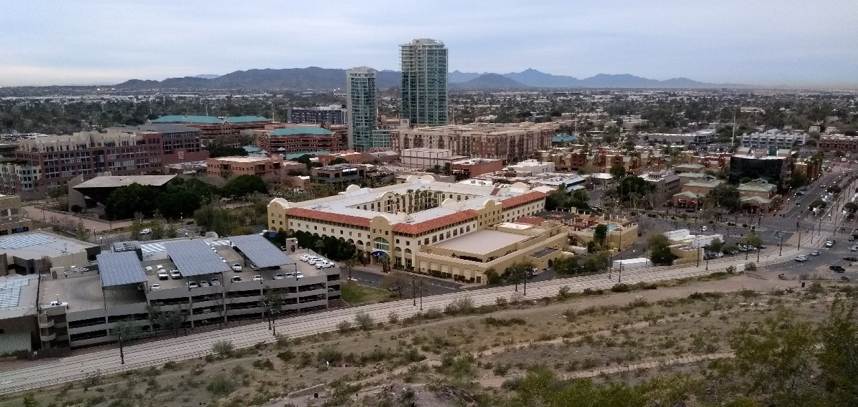
Motivation
- Long-term planning as people are moving
- to a from coast
- to suburbs or city centers
- …
- Assessing impact of these changes before they happen
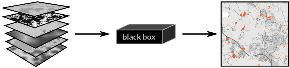
No Room for a Black Box
Can we understand the behavior of the model?Can we make sure it is working as described?
FUTURES
FUTure Urban-Regional
Environment Simulation
(Meentemeyer et al., 2013)
- urban growth model
- patch-based
- stochastic
- accounts for location, quantity, and pattern of change
- positive feedbacks (new development attracts more development)
- allows spatial non-stationarity
FUTURES, A Simplified View
turning green cells into orange cells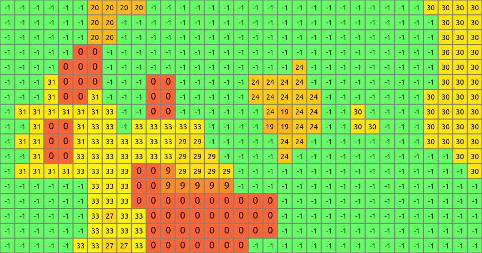
-1: undeveloped, 0: initial development, 1: developed in the first year, …
Modeling framework
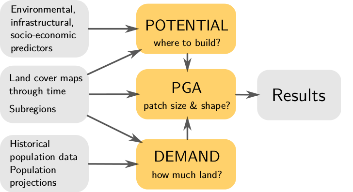
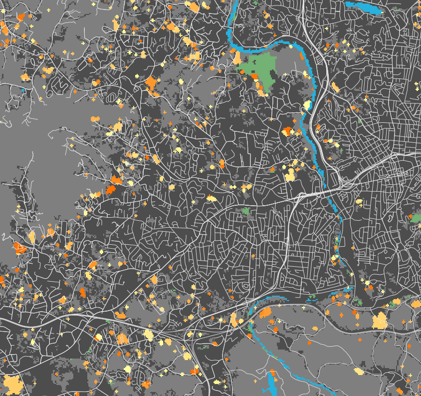
Potential Submodel
- multilevel logistic regression for development suitability accounts for variation among subregions (for example policies in different counties)
- inputs are uncorrelated predictors (distance to roads and development, slope, ...)
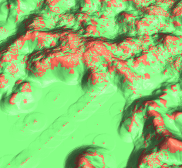
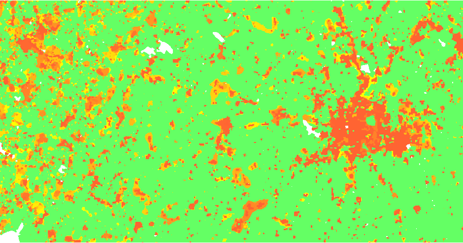
surface: potential, orange: developed areas, green: undeveloped areas
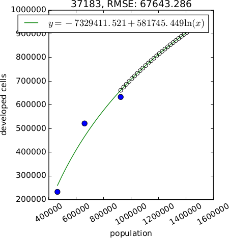
Demand Submodel
- estimates the rate of per capita land consumption for each subregion
- extrapolates between historical changes in population and land conversion
- inputs are historical landuse, population data, population projection
Patch Growing Algorithm (PGA)
- stochastic algorithm
- converts land in discrete patches
- inputs are patch characteristics (distribution of patch sizes and compactness) derived from historical data
FUTURES Prototype
- Private/proprietary
- Only the core of the model formalized in code
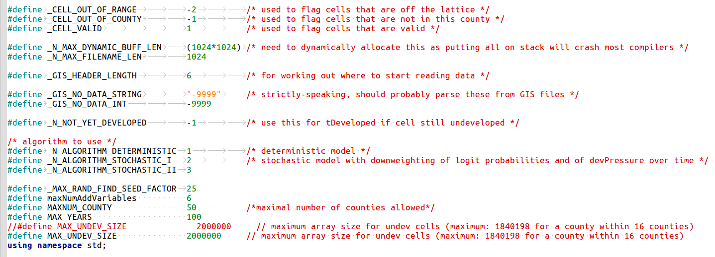
- Poorly documented code with many hardcoded constants
- User interface: configuration file and C code editing
The original paper went through the classic peer-review process and was published in a scientific journal.
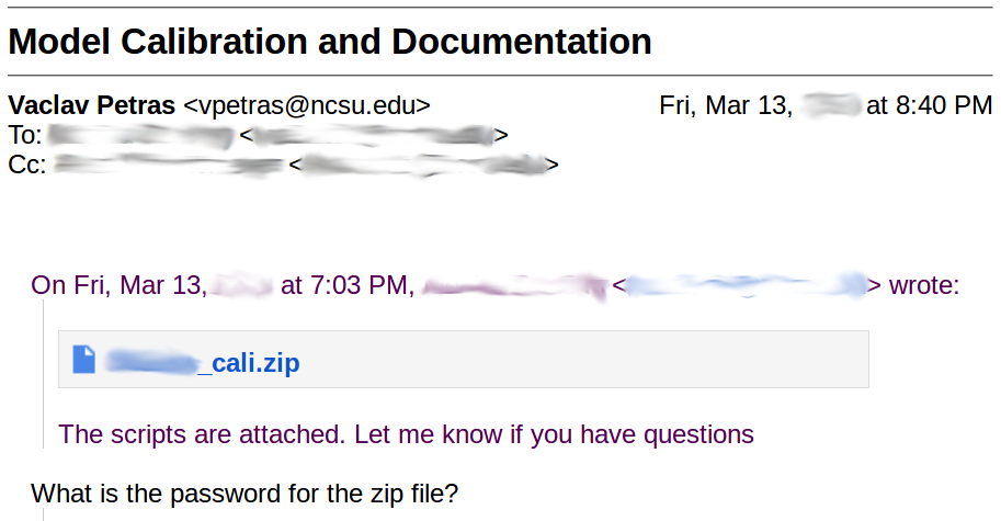
FUTURES Prototype
- Calibration data, tools and documentation distributed in a password-protected ZIP files by email.
Open Source FUTURES
- To pay the technical debt and to go beyond experimental prototype we needed to make FUTURES:
- more efficient and scalable
- as easy to use as possible for a wider audience
- open source, integrated into a larger modeling project, and maintainable in the long run
⇒ new FUTURES GRASS GIS add-on: a set of modules called r.futures
Open science
Image credit: Open Science Logo v2, CC BY-SA 3.0 Greg Emmerich
Why GRASS GIS?
- Advantages for model developers (and all tool/plugin developers):
- modular architecture: modules in C, C++, and Python
- all needed GIS functions at hand
- efficient I/O libraries (several further improvements in GRASS GIS since the decision was made)
- ability to process large datasets
- automatically generated CLI and GUI
- infrastructure for online manual pages
- daily compiled binaries from C/C++ for Windows(thanks to M. Landa, FCE CTU in Prague)
- code in common add-on repository partially maintained by community and core developers
Why GRASS GIS?
- Advantages for model users:
- multiplatform
- graphical user interface
- scriptable (Bash, Python, R, …)
- easy installation from GUI or command line:
g.extension r.futures - more tools available for further analysis and visualization
Why GRASS GIS?
- Advantages for model users:
- spatio-temporal analysis and visualization
Example: Animation tool
r.futures
Information flow diagram for the set of modules implementing FUTURES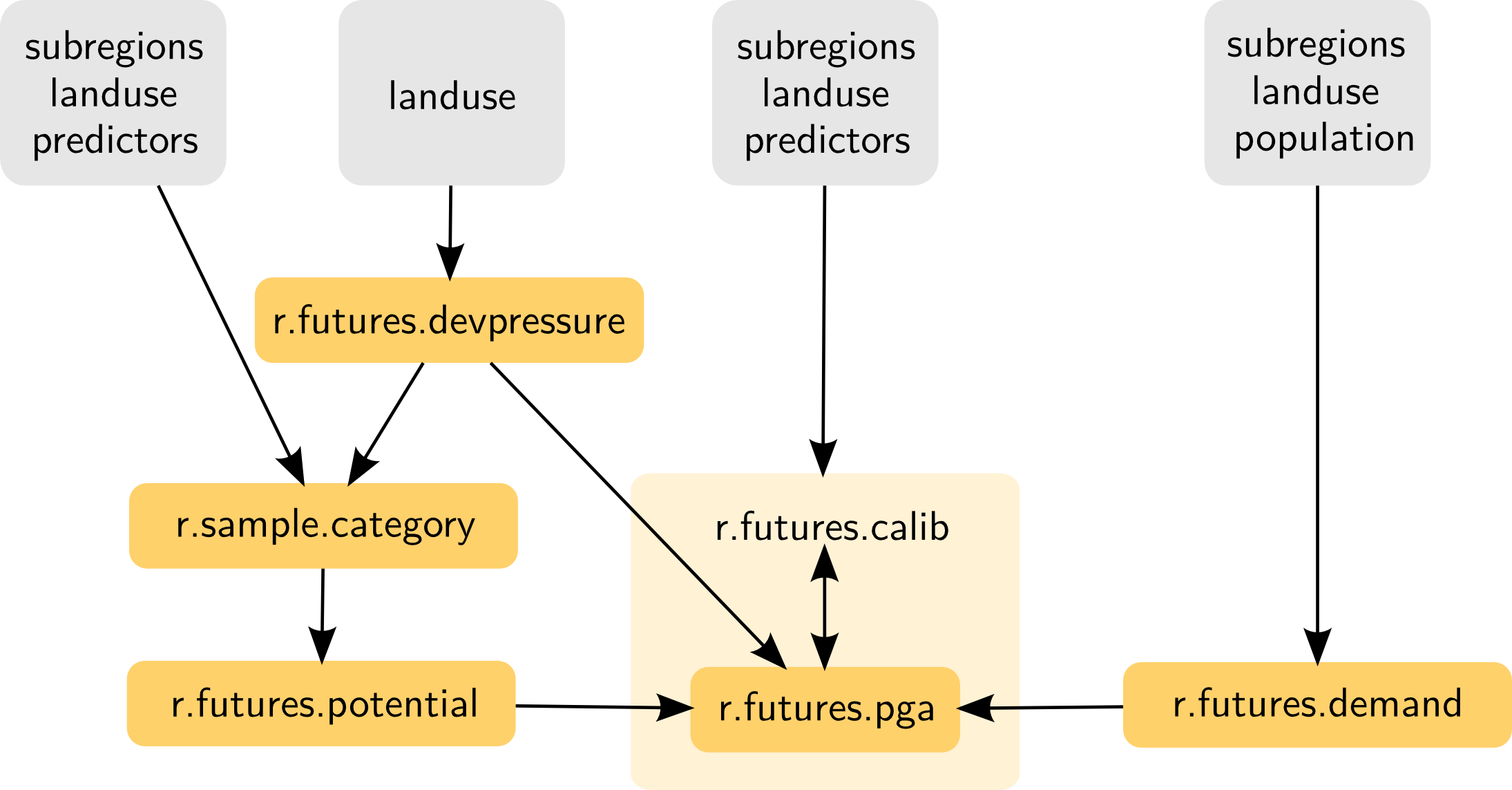
Additionally, r.futures.parallelpga can be used instead of r.futures.pga.
GUI
Graphical User Interface
CLI
Command Line Interface
r.futures.pga -s subregions=counties developed=urban_2011 \
   output=final demand=demand.csv discount_factor=0.1 compactness_mean=0.1 \
   predictors=road_dens_perc,forest_smooth_perc,dist_to_water_km,dist_to_protected_km \
   devpot_params=potential.csv development_pressure=devpressure_0_5 \
   n_dev_neighbourhood=30 gamma=0.5 patch_sizes=patches.txt num_neighbors=4 output=final
TUI
Tangible User Interface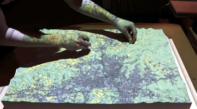
Getting Started: Data
- Import or link data into a GRASS GIS Spatial Database
- Includes reprojection into the same SRS
- Unify resolutions and extents (g.region, r.resamp.stats, …)
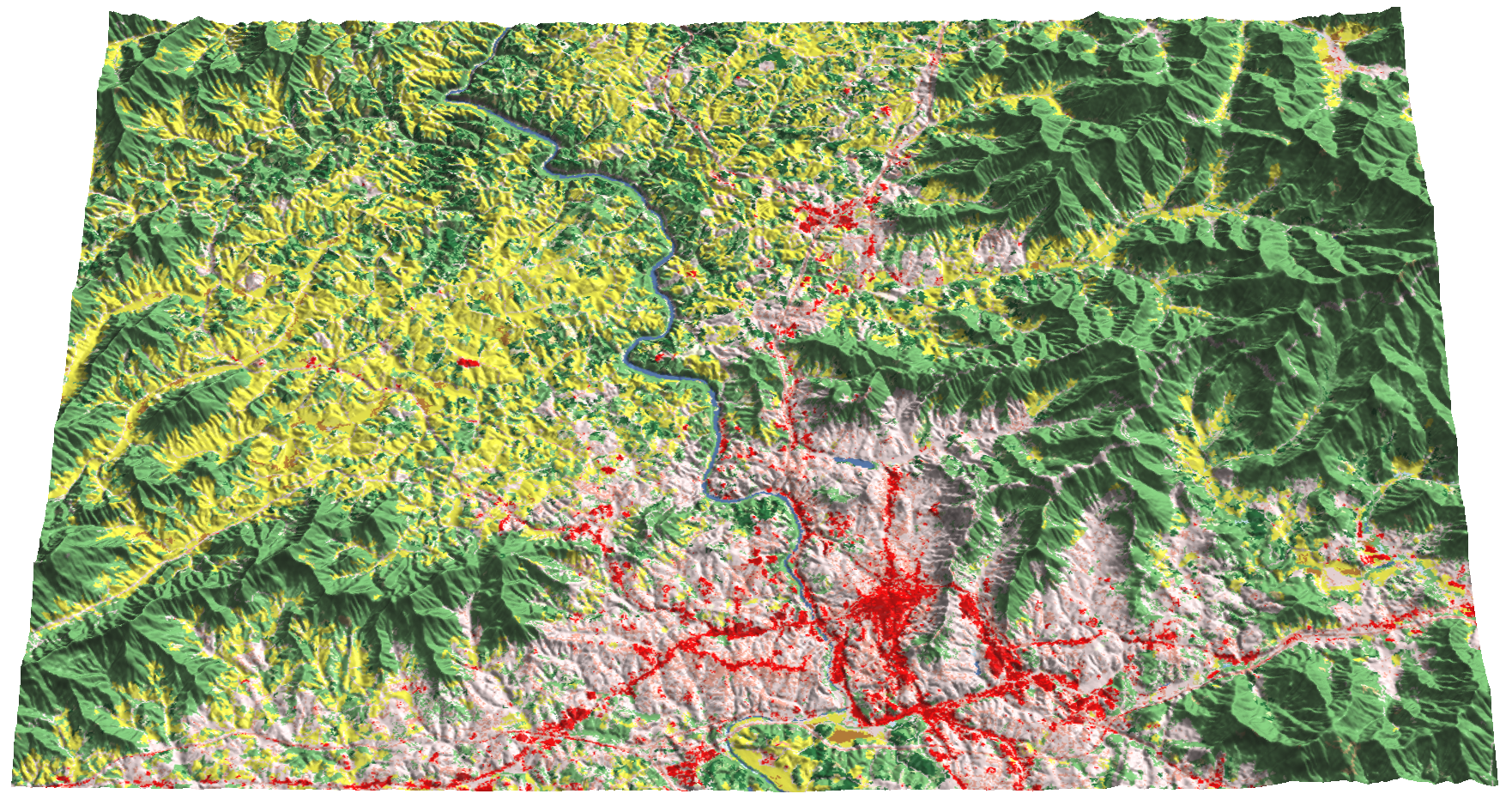
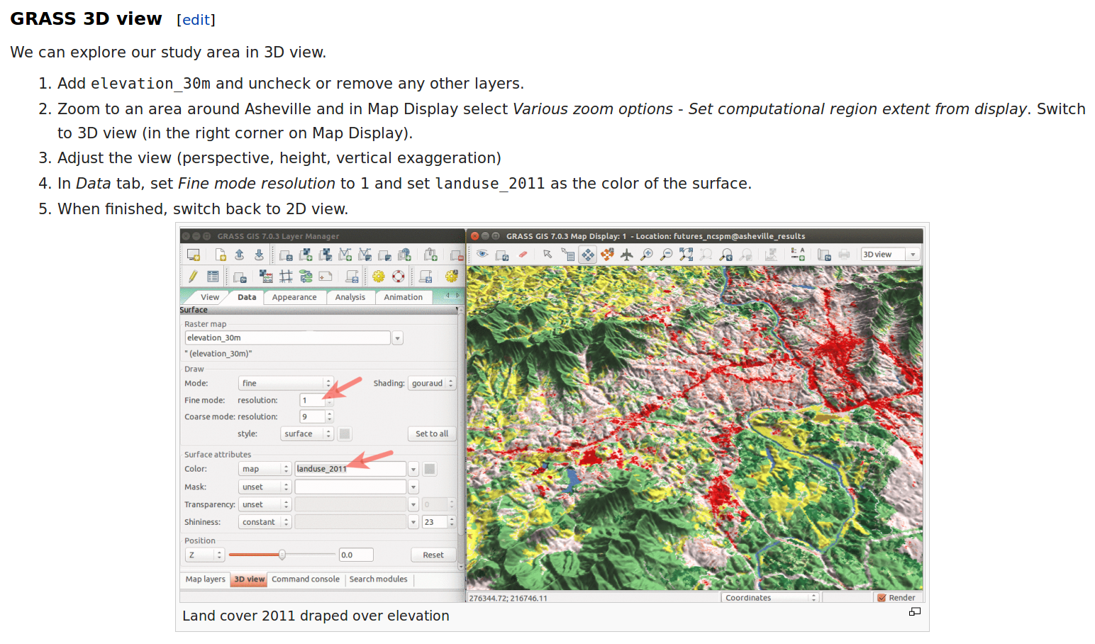
Landuse classes draped over topography (3D view in GRASS GIS)
Getting Started: Calibration
- Potential submodel [calibrated using difference between two years in the past]
- Predictors (distance to water, slope, travel time to city center, …)
- Development pressure (Dynamically modified during the simulation)
- Patch calibration [calibrated using difference between two years in the past]
- Size and shape of patches of new development
- Demand submodel [calibrated using all available past years]
- Equation to relate new development and population growth (past and projected)
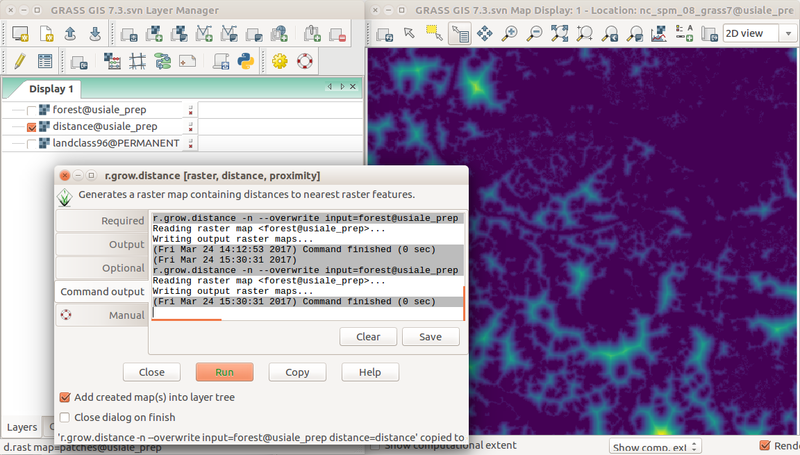
Distance to forest edge computed using r.grow.distance
Getting Started: Scenarios
- stimulus is spatially variable increase potential for development (e.g. zoning)
- constrain_weight is spatially variable limits to development (e.g. city park)
- incentive_power influences infill and sprawl (e.g. government policy)
- change inputs for predictors (e.g. new road) and population growth
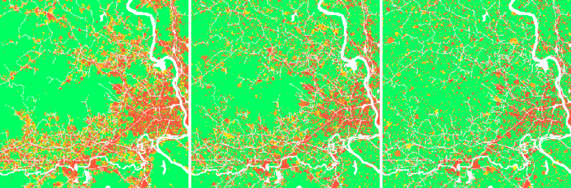 left: infill, middle: status quo, right: sprawl
References
- Meentemeyer, R. K., Tang, W., Dorning, M. A., Vogler, J. B., Cunniffe, N. J. and Shoemaker, D. A., 2013. FUTURES: Multilevel Simulations of Emerging UrbanRural Landscape Structure Using a Stochastic Patch-Growing Algorithm. Annals of the Association of American Geographers 103(4), pp. 785–807.
- Dorning, M. A., Koch, J., Shoemaker, D. A. and Meentemeyer, R. K., 2015. Simulating urbanization scenarios reveals tradeoffs between conservation planning strategies. Landscape and Urban Planning 136, pp. 28–39.
- Pickard, B. R., Van Berkel, D., Petrasova, A. and Meentemeyer, R. K., 2017. Future patterns of urbanization reveal trade-offs among ecosystem services. Landscape Ecology Volume 32, Issue 3, pp 617-634
- Petrasova, A., Petras, V., Van Berkel, D., Harmon, B. A., Mitasova, H., and Meentemeyer, R. K., 2016. Open Source Approach to Urban Growth Simulation. Int. Arch. Photogramm. Remote Sens. Spatial Inf. Sci., XLI-B7, 953-959.
If you can't get to any of these, we can send them to you!
Tutorials
- Tutorial for Triangle (Raleigh, Durham, Chapel Hill) on GRASS GIS Wiki
- Sample dataset for Triangle
- Workshop material for Asheville, NC on GRASS GIS Wiki
- r.futures documentation
Support
In case the tutorials are not enough:
Contact service center at the Center for Geospatial Analytics, NC State University

Highlights
- realistic spatial pattern [Pickard 2017]
- modular (different submodels and data can be plugged in)
- transparent (open source)
- integrated with analytical tools (in GRASS GIS)
- available (open source including its dependencies)
Pickard, B., Gray, J., and Meentemeyer, R.K., 2017. Comparing quantity, allocation and configuration accuracy of multiple land change models. Land 6.3: 52.
Slides: ncsu-landscape-dynamics.github.io/futures-talk
